集合通信总结和 mpi4py 实践
Categories: LLM_Parallel
- 一 集合通信概述
- 二 Broadcast 原理和实践
- 三 Reduce \& AllReduce
- 四 Gather \& AllGather \& AllReduce
- 五 Scatter \& ReduceScatter
- 六 Ring AllReduce
- 七 Alltoall
- 参考资料
一 集合通信概述
1.1 p2p 概述
P2P 是点对点通信,是消息传递系统的基础功能。P2P 支持在进程对之间进行数据传输,一端发送,另一端接收。
集合通信允许在组内多个进程间同时传输数据,即通信参与方是不止 $2$ 个。同时,集合通信还引入了同步点,所有代码在达到同步点后才能继续执行后续的代码。常见的集体通信操作如下:
- 跨所有组成员的屏障同步,这里的成员是指进程。
- 全局通信函数:
Broadcast(广播): 将数据从一个成员广播至组内所有成员。Gather(汇聚):将数据从所有成员收集至组内某个成员。Scatter(发散):将数据从一个成员分散至组内所有成员。
- 求和、求最大值、求最小值等全局规约操作。
1.2 mpi4py 和 torch.distributed
分布式程序都需要一个 launcher,例如 mpiexec、torchrun、ray 等,本文的实例代码使用 mpiexec 和 torchrun 两种。
mpi4py
MPI 是跨语言的并行计算标准,用于在分布式系统中协调多进程通信。在 PyTorch 分布式训练中可作为后端(如 gloo 或 mpi)。mpi4py 是 Python 的 MPI 软件包,为 Python 编程语言提供了 MPI 接口,使任何 Python 程序都能利用多处理器优势。该软件包基于 MPI 规范构建,提供了严格遵循 MPI-2 C++绑定的面向对象接口。
mpi4py 库的安装方式如下:
apt-get update && apt-get install mpich
mpirun --version

pip install mpi4py
pip install torch
mpi4py 基本实例代码如下:
# mpi_hello.py
from mpi4py import MPI

comm = MPI.COMM_WORLD
rank = comm.Get_rank()
size = comm.Get_size()

print(f"Hello from process {rank}/{size}")
运行命令:
mpiexec -n 4 python mpi_hello.py
输出实例:
Hello from process 0/4
Hello from process 1/4
Hello from process 2/4
Hello from process 3/4
torch.distributed
torchrun 是 PyTorch 官方推荐的分布式训练启动工具(取代 torch.distributed.launch),自动处理进程初始化。基本命令格式如下:
torchrun \
    --nnodes={总节点数} \
    --nproc_per_node={每节点GPU数} \
    --node_rank={当前节点ID} \
    --master_addr={主节点IP} \
    --master_port={端口号} \
    YOUR_SCRIPT.py
torchrun 自动注入以下变量,无需手动设置:
- RANK:全局进程 ID
- WORLD_SIZE:总进程数
- LOCAL_RANK:当前节点内的进程 ID
- MASTER_ADDR:主节点 IP
- MASTER_PORT:主节点端口
下述代码是使用分布式数据并行(DistributedDataParallel,简称 DDP)进行简单训练的演示脚本,让每个进程都在单独的 GPU 上执行模型计算。
import torch
import torch.distributed as dist
from torch.nn.parallel import DistributedDataParallel as DDP

def main():
    # 初始化分布式环境,并使用 NCCL 作为通信后端。
    dist.init_process_group(backend="nccl")
    rank = dist.get_rank()
    device = rank

    # 1. 验证数据是否相同
    data = torch.randn(20, 10).to(device)  # 每个进程独立生成随机数据
    print(f"Rank {rank}: Data mean={data.mean().item():.6f}, std={data.std().item():.6f}")

    # 2. 验证模型初始参数是否相同
    model = torch.nn.Linear(10, 10).to(device) # 各进程独立初始化
    print(f"Rank {rank}: Weight mean={model.weight.mean().item():.6f}")

    # 3. DDP包装后参数同步验证
    ddp_model = DDP(model, device_ids=[device]) # DDP同步参数
    print(f"Rank {rank}: DDP Weight mean={ddp_model.module.weight.mean().item():.6f}")

    # 4. 计算输出
    result = ddp_model(data)
    print(f"Rank {rank}: Output mean={result.mean().item():.6f}")

if __name__ == "__main__":
    main()
运行命令如下:
torchrun --nproc_per_node=2 train_torchrun.py
上述代码运行后输出结果如下所示:
[2025-06-28 16:29:17,453] torch.distributed.run: [WARNING]
[2025-06-28 16:29:17,453] torch.distributed.run: [WARNING] *****************************************
[2025-06-28 16:29:17,453] torch.distributed.run: [WARNING] Setting OMP_NUM_THREADS environment variable for each process to be 1 in default, to avoid your system being overloaded, please further tune the variable for optimal performance in your application as needed.
[2025-06-28 16:29:17,453] torch.distributed.run: [WARNING] *****************************************
Rank 1: Data mean=-0.012511, std=1.087953
Rank 1: Weight mean=-0.014889
Rank 0: Data mean=0.059724, std=0.959770
Rank 0: Weight mean=0.000033
Rank 1: DDP Weight mean=0.000033
Rank 0: DDP Weight mean=0.000033
Rank 1: Output mean=-0.065272
Rank 0: Output mean=0.049773
rank0 和 rank1 输出结果不同是因为 torch.randn 使用各进程各自的随机状态生成数据,因为没有显式设置相同的随机种子,所以 rank 0 与 rank 1 产生的 data 自然内容不同。
DDP 的设计就是 “数据并行”:每个进程/GPU 负责一份不同的小批数据,前向结果不要求相同;它只在反向时通信梯度,保证各进程参数同步更新。实例代码中没有反向与优化步骤,只做一次前向打印,所以看到输出差异是正常的。
1.3 mpi4py.MPI.Comm 类总结
mpi4py.MPI.Comm 类是 MPI(Message Passing Interface)在 Python 中的核心通信器类,用于管理进程组间的通信上下文。MPI 所有点对点 / 集体通信均以 Comm 为起点调用。典型实例:
MPI.COMM_WORLD:包含启动作业的全部进程MPI.COMM_SELF:仅包含自身- 派生子通信域:由 Comm.Split、Comm.Create、Cartcomm、Graphcomm 等方法生成
核心属性
| 方法/属性 | 描述 | 示例 |
|---|---|---|
Get_size() |
获取通信器(域)包含的进程总数 | size = comm.Get_size() |
Get_rank() |
获取当前进程在组内的排名(rank) | rank = comm.Get_rank() |
Get_group() |
获取关联的进程组对象 | group = comm.Get_group() |
Get_name() |
获取通信器名称 | name = comm.Get_name() |
主要实例方法(按功能归类)
A) 点对点通信
- send(obj, dest, tag=0): 以标准模式发送。
- recv(source=MPI.ANY_SOURCE, tag=MPI.ANY_TAG, status=None)
- isend / irecv:立即返回 Request,可与 Wait/Test 配合
- sendrecv(sendobj, dest, sendtag, recvobj, source, recvtag, status=None)
- ssend / bsend:同步或缓冲发送
B) 集体通信
| 方法 | 描述 |
|---|---|
Bcast(buf[, root]) |
将数据从根进程广播至所有其他进程 |
Scatter(sendbuf, recvbuf[, root]) |
根进程分发数据 |
Gather(sendbuf, recvbuf[, root]) |
将数据从所有进程收集到一个进程(根进程) |
Allgather(sendbuf, recvbuf) |
所有进程收集所有数据 |
Reduce(sendbuf, recvbuf[, op, root]) |
归约操作到根进程 |
Allreduce(sendbuf, recvbuf[, op]) |
全归约操作(所有进程获结果) |
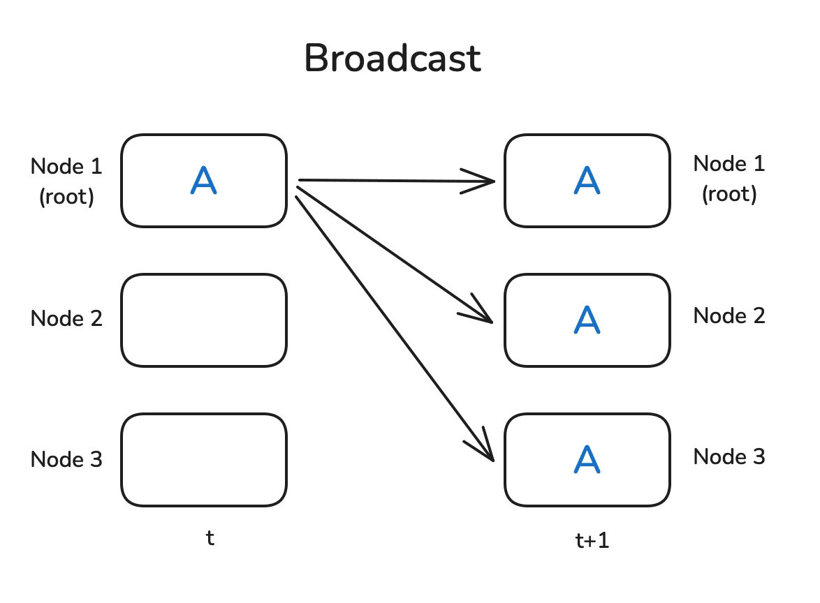
二 Broadcast 原理和实践
Broadcast 广播将一个进程(或节点)中的数据发送到所有其他进程(节点)。通常用于将一个进程的消息或数据复制到所有参与者。
Broadcast 操作的 mpi4py 实例代码:
from mpi4py import MPI
import numpy as np

comm = MPI.COMM_WORLD
rank = comm.Get_rank()
size = comm.Get_size()

def demo_broadcast():
    """
    Broadcast:root 进程准备一份数据,把它广播给通信域内所有进程。
    """
    if rank == 0:
        data = {"msg": "Hello", "vec": np.arange(4)}
        print(f"[BCAST] Rank 0 初始化数据 -> {data}")
    else:
        data = None                 # 非 root 必须占位
    data = comm.bcast(data, root=0) # 广播
    print(f"[BCAST] Rank {rank} 收到数据 -> {data}")

if __name__ == "__main__":
    if rank == 0:
        print(f"=== 进程总数: {size} ===\n")

    comm.Barrier()   # 让所有进程同步后再开始演示
    if rank == 0: print("\n*** Broadcast 演示 ***")
    demo_broadcast()
torch.distributed 的广播示例代码很简单,流程如下:
- 首先,通过
dist.initi_process_group初始化一个进程组,用于设置通信后端(如nccl),并设置worker工作进程(节点)数量,并为每个工作进程分配一个等级(通过dist.get_rank获得)。 - 然后,创建一个在
rank=0上具有非零值的张量,其他worker创建充满零的张量,通过dist.broadcast(tensor, src=0)将 rank 0 上的张量分发给所有其他进程。
完整代码如下所示:
import torch
import torch.distributed as dist

def init_process():
    dist.init_process_group(backend='nccl')
    torch.cuda.set_device(dist.get_rank())

def example_broadcast():
    if dist.get_rank() == 0:
        tensor = torch.tensor([1, 2, 3, 4, 5], dtype=torch.float32).cuda()
    else:
        tensor = torch.zeros(5, dtype=torch.float32).cuda()
    print(f"Before broadcast on rank {dist.get_rank()}: {tensor}")
    dist.broadcast(tensor, src=0)
    print(f"After broadcast on rank {dist.get_rank()}: {tensor}")

init_process()
example_broadcats()
运行命令和输出结果如下所示:
torchrun --nproc_per_node=2 dist_op.py

Before broadcast on rank 0: tensor([1., 2., 3., 4., 5.], device='cuda:0')
Before broadcast on rank 1: tensor([0., 0., 0., 0., 0.], device='cuda:1')

After broadcast on rank 0: tensor([1., 2., 3., 4., 5.], device='cuda:0')
After broadcast on rank 1: tensor([1., 2., 3., 4., 5.], device='cuda:1')
三 Reduce & AllReduce
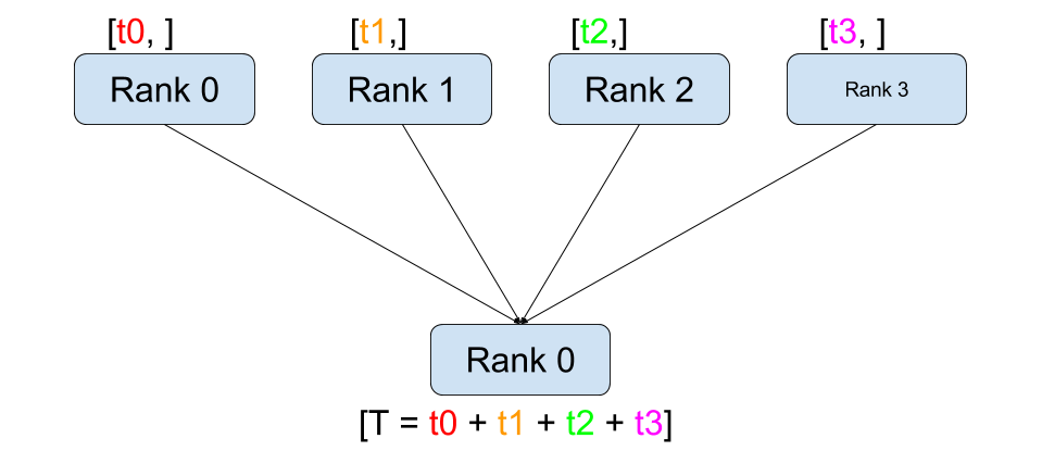
Reduce 是分布式数据处理中的一种基础模式,其核心思想是在各个节点上执行某个函数 f()(例如求和或平均),并将数据进行合并。
Reduce: 合并结果只发送给根节点;AllReduce: 结果则会同步到所有节点。
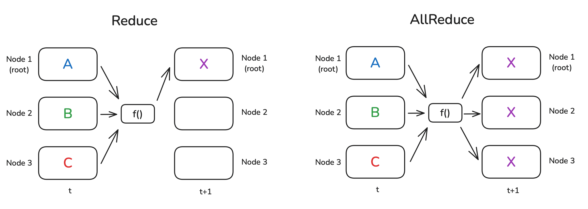
看上图,f() 函数是悬空的,毕竟,并没有哪个节点能“凭空”完成整个操作。通常,各个节点会进行局部计算,并按照环形或树状结构协同完成任务。举个例子:假设每个节点上都有一个数字,我们要计算它们的总和,并且节点之间按环状相连。
Ring(环)AllReduce 原理、可视化和通信量分析可以参考我的另一篇文章。
下述是一个简单的 Reduce 操作示例,用于对多个张量进行求和。通过设置 op=dist.ReduceOp.SUM 来指定使用的归约操作。
def example_reduce():
    tensor = torch.tensor([dist.get_rank() + 1] * 5, dtype=torch.float32).cuda()
    print(f"Before reduce on rank {dist.get_rank()}: {tensor}")
    dist.reduce(tensor, dst=0, op=dist.ReduceOp.SUM)
    print(f"After reduce on rank {rank}: {tensor}")

init_process()
example_reduce()
运行命令和输出结果如下所示。注意,因为是 reduce 操作,所以仅更新 dst(0)节点上的张量。
torchrun --nproc_per_node=2 dist_reduce.py

Before reduce on rank 0: tensor([1., 1., 1., 1., 1.], device='cuda:0')
Before reduce on rank 1: tensor([2., 2., 2., 2., 2.], device='cuda:1')

After reduce on rank 0: tensor([3., 3., 3., 3., 3.], device='cuda:0')
After reduce on rank 1: tensor([2., 2., 2., 2., 2.], device='cuda:1')
同样的,按如下方式执行 AllReduce 操作(呜呜指定 dst)
def example_all_reduce():
    tensor = torch.tensor([dist.get_rank() + 1] * 5, dtype=torch.float32).cuda()
    print(f"Before all_reduce on rank {dist.get_rank()}: {tensor}")
    dist.all_reduce(tensor, op=dist.ReduceOp.SUM)
    print(f"After all_reduce on rank {dist.get_rank()}: {tensor}")

init_process()
example_all_reduce()
运行命令和输出结果如下所示:
torchrun --nproc_per_node=2 dist_allreduce.py

Before reduce on rank 0: tensor([1., 1., 1., 1., 1.], device='cuda:0')
Before reduce on rank 1: tensor([2., 2., 2., 2., 2.], device='cuda:1')

After reduce on rank 0: tensor([3., 3., 3., 3., 3.], device='cuda:0')
After reduce on rank 0: tensor([3., 3., 3., 3., 3.], device='cuda:0')
四 Gather & AllGather & AllReduce
4.1 Gather & AllGather 原理和实践
Gather 和 AllGather 操作本质上与 Broadcast 类似,都是在各个节点之间分发数据且不改变数据本身。但不同的是,Broadcast 是从某一个节点向所有节点广播同一个数据,而 Gather 和 AllGather 的场景中,每个节点都有一份独立的数据块:
Gather: 会把这些数据收集到一个指定节点上;AllGather: 则是让所有节点最终都拥有全部的数据。
示意图如下所示:
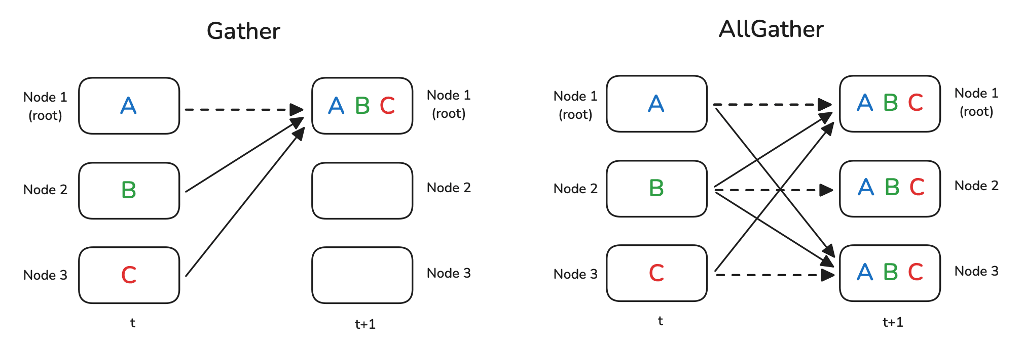
虚线表示某些数据实际上根本没有移动(因为它已经存在于节点上)。
在执行 Gather 操作时,我们需要准备一个容器对象用于存放收集到的张量,在下面的示例中,就是 gather_list 对象。
dist.gather 示例代码如下所示:
def example_gather():
    tensor = torch.tensor([dist.get_rank() + 1] * 5, dtype=torch.float32).cuda()
    if dist.get_rank() == 0:
        gather_list = [
            torch.zeros(5, dtype=torch.float32).cuda()
            for _ in range(dist.get_world_size())
            ]
    else:
        gather_list = None
    print(f"Before gather on rank {dist.get_rank()}: {tensor}")
    dist.gather(tensor, gather_list, dst=0)
    if dist.get_rank() == 0:
        print(f"After gather on rank 0: {gather_list}")

init_process()
example_gather()
输出结果中 gather_list 确实包含所有 rank 的张量:
Before gather on rank 0: tensor([1., 1., 1., 1., 1.], device='cuda:0')
Before gather on rank 1: tensor([2., 2., 2., 2., 2.], device='cuda:1')

After gather on rank 0: [tensor([1., 1., 1., 1., 1.], device='cuda:0'),
                         tensor([2., 2., 2., 2., 2.], device='cuda:0')]
对于 AllGather 示例,每个 rank 都要预先准备一个用于接收所有结果的占位容器 gather_list。dist.all_gather 示例代码如下所示:
def example_allgather():
    tensor = torch.tensor([dist.get_rank() + 1] * 5, dtype=torch.float32).cuda()
    gather_list = [
        torch.zeros(5, dtype=torch.float32).cuda()
        for _ in range(dist.get_world_size())
        ]
    print(f"Before gather on rank {dist.get_rank()}: {tensor}")
    dist.all_gather(tensor, gather_list)
    print(f"After gather on rank 0: {gather_list}")

init_process()
example_allgather()
从输出结果可以看出,每个节点现在都有所有数据:
Before all_gather on rank 0: tensor([1., 1., 1., 1., 1.], device='cuda:0')
Before all_gather on rank 1: tensor([2., 2., 2., 2., 2.], device='cuda:1')

After all_gather on rank 0: [tensor([1., 1., 1., 1., 1.], device='cuda:0'),
                             tensor([2., 2., 2., 2., 2.], device='cuda:0')]
After all_gather on rank 1: [tensor([1., 1., 1., 1., 1.], device='cuda:1'),
                             tensor([2., 2., 2., 2., 2.], device='cuda:0')]
Gather(收集)的“反操作”是什么呢?假设现在所有数据都集中在一个节点上:
- 如果希望将这些数据切分并分发给各个节点,则可以使用
Scatter操作; - 如果在分发前还需要先对数据进行归约处理,那就可以采用
ReduceScatter模式。
4.2 All-Gather 和 All-Reduce
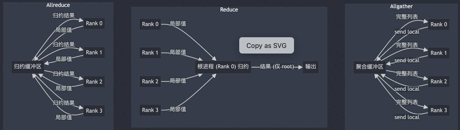
Allgather 是 Gather 的进阶版。All Gather 操作是将所有进程中的数据汇聚到每个进程中。每个进程不仅接收来自根进程的数据,还接收来自其他所有进程的数据。
Reduce 操作将多个进程中的数据通过某种运算(如求和、取最大值等)整合成一个结果,并将该结果发送到一个指定的根进程。
All Reduce 操作是将所有进程中的数据进行归约运算,并将结果发送到所有进程。每个进程都能获得归约后的结果。
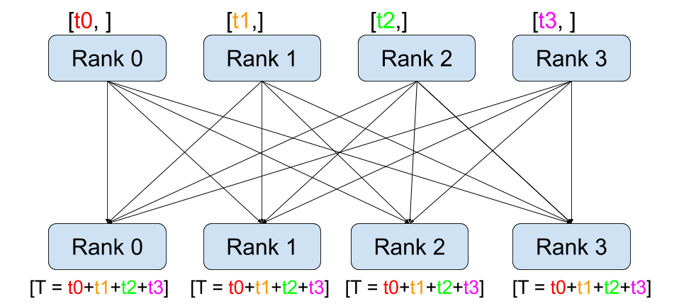
三者对比图如下所示:
三者实例代码如下所示:
# collective_ops.py
from mpi4py import MPI
import numpy as np

comm = MPI.COMM_WORLD
rank, size = comm.Get_rank(), comm.Get_size()

def demo_allgather():
    """
    每个进程发出局部向量,所有进程都得到完整列表
    """
    local_vec = np.arange(rank*3, rank*3 + 3, dtype='i')  # eg Rank2->[6 7 8]
    gathered = comm.allgather(local_vec)
    print(f"[ALLGATHER] Rank {rank}: local={local_vec} → gathered={gathered}")

def demo_reduce():
    """
    将标量归约到 root;这里只做求和
    """
    local_val = (rank + 1) ** 2          # 1,4,9,16
    total = comm.reduce(local_val, op=MPI.SUM, root=0)
    if rank == 0:
        print(f"\n[REDUCE] 汇总结果 (sum) = {total}")  # 1+4+9+16=30

def demo_allreduce():
    """
    所有进程都同时得到归约值;这里做 max
    """
    local_val = (rank + 1) * 2           # 2,4,6,8
    global_max = comm.allreduce(local_val, op=MPI.MAX)
    print(f"[ALLREDUCE] Rank {rank}: local={local_val}, global_max={global_max}")

if __name__ == "__main__":
    if rank == 0:
        print(f"\n=== 进程总数: {size} ===\n")

    comm.Barrier();  demo_allgather()
    comm.Barrier();  demo_reduce()
    comm.Barrier();  demo_allreduce()
运行命令:
mpiexec -np 4 --allow-run-as-root python mpi4py_allreduce.py
输出结果:
=== 进程总数: 4 ===

[ALLGATHER] Rank 0: local=[0 1 2] → gathered=[array([0, 1, 2], dtype=int32), array([3, 4, 5], dtype=int32), array([6, 7, 8], dtype=int32), array([ 9, 10, 11], dtype=int32)]
[ALLGATHER] Rank 2: local=[6 7 8] → gathered=[array([0, 1, 2], dtype=int32), array([3, 4, 5], dtype=int32), array([6, 7, 8], dtype=int32), array([ 9, 10, 11], dtype=int32)]
[ALLGATHER] Rank 1: local=[3 4 5] → gathered=[array([0, 1, 2], dtype=int32), array([3, 4, 5], dtype=int32), array([6, 7, 8], dtype=int32), array([ 9, 10, 11], dtype=int32)]
[ALLGATHER] Rank 3: local=[ 9 10 11] → gathered=[array([0, 1, 2], dtype=int32), array([3, 4, 5], dtype=int32), array([6, 7, 8], dtype=int32), array([ 9, 10, 11], dtype=int32)]

[REDUCE] 汇总结果 (sum) = 30
[ALLREDUCE] Rank 0: local=2, global_max=8
[ALLREDUCE] Rank 2: local=6, global_max=8
[ALLREDUCE] Rank 3: local=8, global_max=8
[ALLREDUCE] Rank 1: local=4, global_max=8
五 Scatter & ReduceScatter
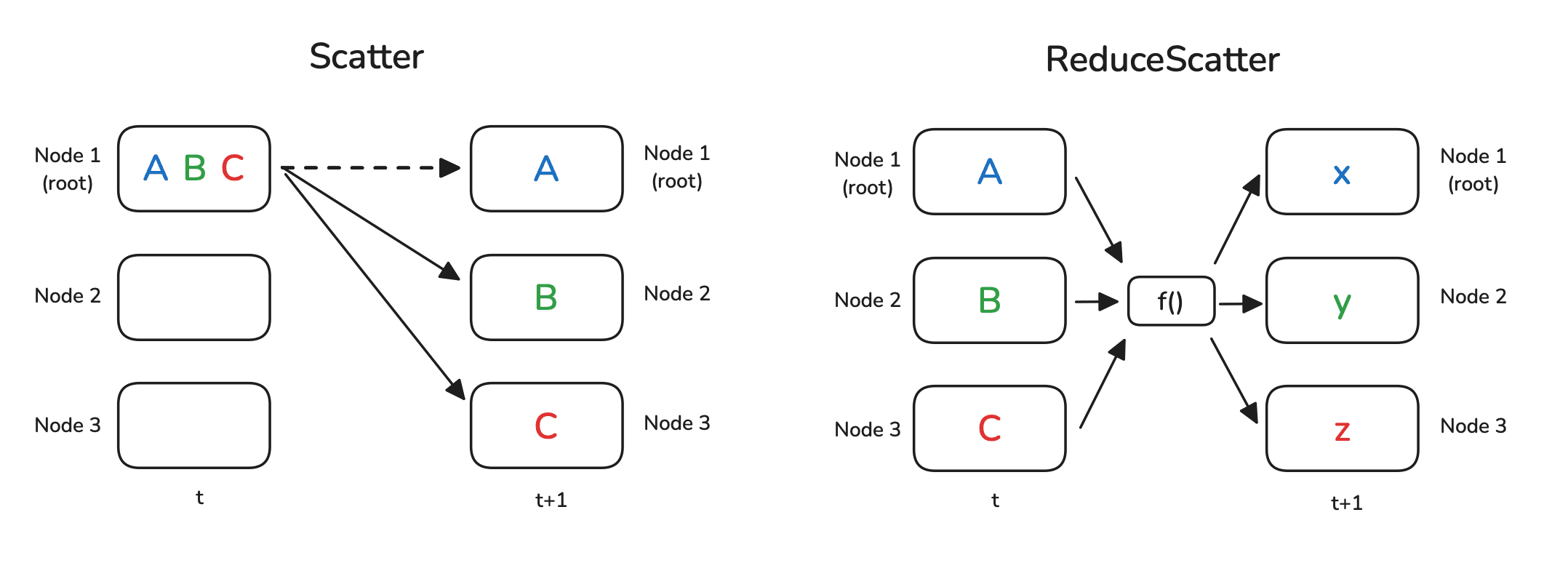
Scatter 操作的作用是将一个节点上的数据切片并分发给所有其他节点,每个节点接收到数据的一部分。
ReduceScatter 和 AllReduce 类似,都会对所有节点上的数据执行某种操作(如求和)。但不同的是:
- 在 AllReduce 中,每个节点最终会接收到完整的归约结果;
- 而在 ReduceScatter 中,每个节点只接收归约结果的一部分切片。
Scatter 是 Gather 的反向过程,因此需要准备的是一个源张量列表,表示要分发出去的数据,而不是用于接收的目标列表。同时,还需要通过 src 参数指定数据来源的节点。
import torch
import torch.distributed as dist

def init_process():
    dist.init_process_group(backend='nccl')
    torch.cuda.set_device(dist.get_rank())

def example_scatter():
    if dist.get_rank() == 0:
        scatter_list = [
            torch.tensor([i + 1] * 5, dtype=torch.float32).cuda()
            for i in range(dist.get_world_size())
            ]
        print(f"Rank 0: Tensor to scatter: {scatter_list}")
    else:
        scatter_list = None
    tensor = torch.empty(5, dtype=torch.float32).cuda()

    print(f"Before scatter on rank {dist.get_rank()}: {tensor}")
    dist.scatter(tensor, scatter_list, src=0)
    print(f"After scatter on rank {dist.get_rank()}: {tensor}")

init_process()
example_scatter()
零(空)张量被 scatter_list 的内容填充:
torchrun --nproc_per_node=2 dist_scater.py

Rank 0: Tensor to scatter: [tensor([1., 1., 1., 1., 1.], device='cuda:0'),
                            tensor([2., 2., 2., 2., 2.], device='cuda:0')]
Before scatter on rank 0: tensor([0., 0., 0., 0., 0.], device='cuda:0')
Before scatter on rank 1: tensor([0., 0., 0., 0., 0.], device='cuda:1')
After scatter on rank 0: tensor([1., 1., 1., 1., 1.], device='cuda:0')
After scatter on rank 1: tensor([2., 2., 2., 2., 2.], device='cuda:1')
为了更好地演示 ReduceScatter 的工作方式,我们先在每个节点上生成一组更有规律的数据:每个节点创建一个包含两个元素向量的列表,数值由幂函数和与 rank 相关的偏移量计算得出。
import torch
import torch.distributed as dist

def init_process():
    dist.init_process_group(backend='nccl')
    torch.cuda.set_device(dist.get_rank())

def example_reduce_scatter():
    rank = dist.get_rank()
    world_size = dist.get_world_size()
    input_tensor = [
        torch.tensor([(rank + 1) * i for i in range(1, 3)], dtype=torch.float32).cuda()**(j+1)
        for j in range(world_size)
        ]
    output_tensor = torch.zeros(2, dtype=torch.float32).cuda()
    print(f"Before ReduceScatter on rank {rank}: {input_tensor}")
    dist.reduce_scatter(output_tensor, input_tensor, op=dist.ReduceOp.SUM)
    print(f"After ReduceScatter on rank {rank}: {output_tensor}")

init_process()
example_reduce_scatter()
从打印结果可以看出,每个节点生成的数据都符合预期的规律。同时,ReduceScatter 的行为也非常清晰:第 0 个节点收到了所有节点中第一个张量的求和结果,第 1 个节点收到了所有节点中第二个张量的求和结果,更多节点也是依此类推。
torchrun --nproc_per_node=2 dist_reduce_scater.py
Before ReduceScatter on rank 0: [tensor([1., 2.], device='cuda:0'), tensor([1., 4.], device='cuda:0')]
Before ReduceScatter on rank 1: [tensor([2., 4.], device='cuda:1'), tensor([4., 16.], device='cuda:1')]

After ReduceScatter on rank 0: tensor([3., 6.], device='cuda:0')
After ReduceScatter on rank 1: tensor([5., 20.], device='cuda:1')
六 Ring AllReduce
Ring AllReduce 是一种专为分布式系统可扩展性设计的高效 AllReduce 实现方案。它避免了所有 GPU 之间直接通信所带来的网络瓶颈,转而将 AllReduce 拆分为两个步骤:ReduceScatter 和 AllGather。其工作机制如下:
✅ ReduceScatter 阶段
- 每个 GPU 会将自己的数据(例如梯度)等分为 $N$ 块($N$ 是总
GPU数)。 - 然后它将其中一块数据发送给右侧的邻居,同时接收来自左侧邻居的一块数据。
- 每当收到一块数据时,它就与自己对应的本地块执行求和(reduce)。
- 这个过程会沿着环形结构持续传递,直到每个 GPU 得到一块已经在所有设备上累加过的结果。
✅ AllGather 阶段
- 此时,每个 GPU 拥有了一块完整求和后的数据。接下来需要交换数据,使每个 GPU 拥有全部的块。
- 每轮中,GPU 把自己已有的块发送给邻居,同时接收另一个邻居的块。
- 经过 $N−1$ 轮交换后,所有 GPU 都拥有了所有的数据块,从而完成了完整的 AllReduce。
下图演示了这个过程:我们用 5 个 GPU,每个拥有长度为 5 的张量为例。第一幅动画展示的是 ReduceScatter 阶段,在这一阶段结束时,每个 GPU 拿到一块经过归约处理的数据块(图中以橙色矩形标示)。
下面的动画显示了 AllGather 步骤,其中,在最后,每个 GPU 都会获取 AllReduce 作的完整结果。
6.1 Ring-AllReduce 通信量分析
可能已经注意到,在 ReduceScatter 和 AllGather 两个阶段中,每个 GPU 都要进行 $N - 1$ 次发送和接收操作(共计 $2 \times (N - 1)$ 次通信),其中 $N$ 是 GPU 数量。每次传输的内容为 $\frac{K}{N}$ 个元素,$K$ 表示总共需要归约的参数数量。
因此,每个 GPU 总共需要传输的数据量是:$2 \times (N - 1) \times \frac{K}{N}$,当 GPU 数量 N 较大时,这一公式近似为:$2 \times K$。也就是说,每个 GPU 在整个 Ring AllReduce 过程中,总共传输了大约两倍于模型参数数量的数据。
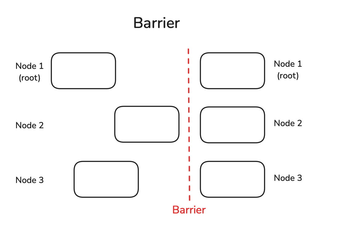
6.2 Barrier 概述
Barrier(同步屏障) 是一种用于协调所有节点的简单同步机制。它会阻塞程序执行,直到所有节点都到达这一点为止,之后所有节点才能继续执行后续计算。
def example_barrier():
    rank = dist.get_rank()
    t_start = time.time()
    print(f"Rank {rank} sleeps {rank} seconds.")
    time.sleep(rank)  # Simulate different processing times
    dist.barrier()
    print(f"Rank {rank} after barrier time delta: {time.time()-t_start:.4f}")

init_process()
example_barrier()
虽然第一个 rank 并没有真正休眠,但因为用上了 dist.barrier(),所以仍然等了 2 秒才通过同步屏障(Barrier)。
Rank 0 sleeps 0 seconds.
Rank 1 sleeps 1 seconds.

Rank 0 after barrier time delta: 2.0025
Rank 1 after barrier time delta: 2.0025
七 Alltoall
7.1 Scatter 和 Gather示例代码
Broadcast、Scatter、Gather 的运行实例代码如下所示:
# comm_ops.py
from mpi4py import MPI
import numpy as np

comm = MPI.COMM_WORLD
rank = comm.Get_rank()
size = comm.Get_size()

def demo_broadcast():
    """
    Broadcast:root 进程准备一份数据,把它广播给通信域内所有进程。
    """
    if rank == 0:
        data = {"msg": "Hello", "vec": np.arange(4)}
        print(f"[BCAST] Rank 0 初始化数据 -> {data}")
    else:
        data = None                 # 非 root 必须占位
    data = comm.bcast(data, root=0) # 广播
    print(f"[BCAST] Rank {rank} 收到数据 -> {data}")

def demo_scatter():
    """
    Scatter:root 进程按进程数把一个可迭代对象切块,分别送到各进程。
    最终每个进程仅拿到自己的“那一块”。
    """
    if rank == 0:
        big_array = np.arange(size * 3, dtype='i')   # 举例:总长度 = 进程数 × 3
        chunks = np.split(big_array, size)           # 均匀切成 size 份
        print(f"[SCATTER] Rank 0 切割后 chunks = {chunks}")
    else:
        chunks = None
    local_arr = comm.scatter(chunks, root=0)  # 本进程获得一个形状 (3,) 的子数组
    print(f"[SCATTER] Rank {rank} 拿到 {local_arr}, 平均={local_arr.mean():.1f}")

def demo_gather(local_data):
    """
    Gather:把各进程局部结果收集到 root 进程,root 获得列表,其他进程得 None
    Allgather:所有进程都得到完整列表
    """
    gathered = comm.gather(local_data, root=0)
    if rank == 0:
        print(f"[GATHER] Root 收到来自所有进程的数据 -> {gathered}\n")

    gathered_all = comm.allgather(local_data)
    print(f"[ALLGATHER] Rank {rank} 收到完整数据列表 -> {gathered_all}")

if __name__ == "__main__":
    if rank == 0:
        print(f"\n=== 进程总数: {size} ===")

    comm.Barrier()
    if rank == 0: print("\n*** Broadcast 演示 ***")
    demo_broadcast()

    comm.Barrier()
    if rank == 0: print("\n*** Scatter + Gather 演示 ***")
    local = demo_scatter()

    comm.Barrier()
    demo_gather(local)
按下述命令运行代码:
mpiexec -np 4 --allow-run-as-root python mpi4py_bcast.py
运行后输出结果如下所示:
=== 进程总数: 4 ===

*** Broadcast 演示 ***
[BCAST] Rank 0 初始化数据 -> {'msg': 'Hello', 'vec': array([0, 1, 2, 3])}
[BCAST] Rank 0 收到数据 -> {'msg': 'Hello', 'vec': array([0, 1, 2, 3])}
[BCAST] Rank 1 收到数据 -> {'msg': 'Hello', 'vec': array([0, 1, 2, 3])}
[BCAST] Rank 2 收到数据 -> {'msg': 'Hello', 'vec': array([0, 1, 2, 3])}
[BCAST] Rank 3 收到数据 -> {'msg': 'Hello', 'vec': array([0, 1, 2, 3])}

*** Scatter + Gather 演示 ***
[SCATTER] Rank 0 切割后 chunks = [array([0, 1, 2], dtype=int32), array([3, 4, 5], dtype=int32), array([6, 7, 8], dtype=int32), array([ 9, 10, 11], dtype=int32)]
[SCATTER] Rank 1 拿到 [3 4 5], 平均=4.0
[SCATTER] Rank 0 拿到 [0 1 2], 平均=1.0
[SCATTER] Rank 3 拿到 [ 9 10 11], 平均=10.0
[SCATTER] Rank 2 拿到 [6 7 8], 平均=7.0
[GATHER] Root 收到来自所有进程的数据 -> [array([0, 1, 2], dtype=int32), array([3, 4, 5], dtype=int32), array([6, 7, 8], dtype=int32), array([ 9, 10, 11], dtype=int32)]

[ALLGATHER] Rank 0 收到完整数据列表 -> [array([0, 1, 2], dtype=int32), array([3, 4, 5], dtype=int32), array([6, 7, 8], dtype=int32), array([ 9, 10, 11], dtype=int32)]
[ALLGATHER] Rank 2 收到完整数据列表 -> [array([0, 1, 2], dtype=int32), array([3, 4, 5], dtype=int32), array([6, 7, 8], dtype=int32), array([ 9, 10, 11], dtype=int32)]
[ALLGATHER] Rank 3 收到完整数据列表 -> [array([0, 1, 2], dtype=int32), array([3, 4, 5], dtype=int32), array([6, 7, 8], dtype=int32), array([ 9, 10, 11], dtype=int32)]
[ALLGATHER] Rank 1 收到完整数据列表 -> [array([0, 1, 2], dtype=int32), array([3, 4, 5], dtype=int32), array([6, 7, 8], dtype=int32), array([ 9, 10, 11], dtype=int32)]
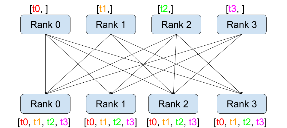
8.2 Alltoall 可视化和示例
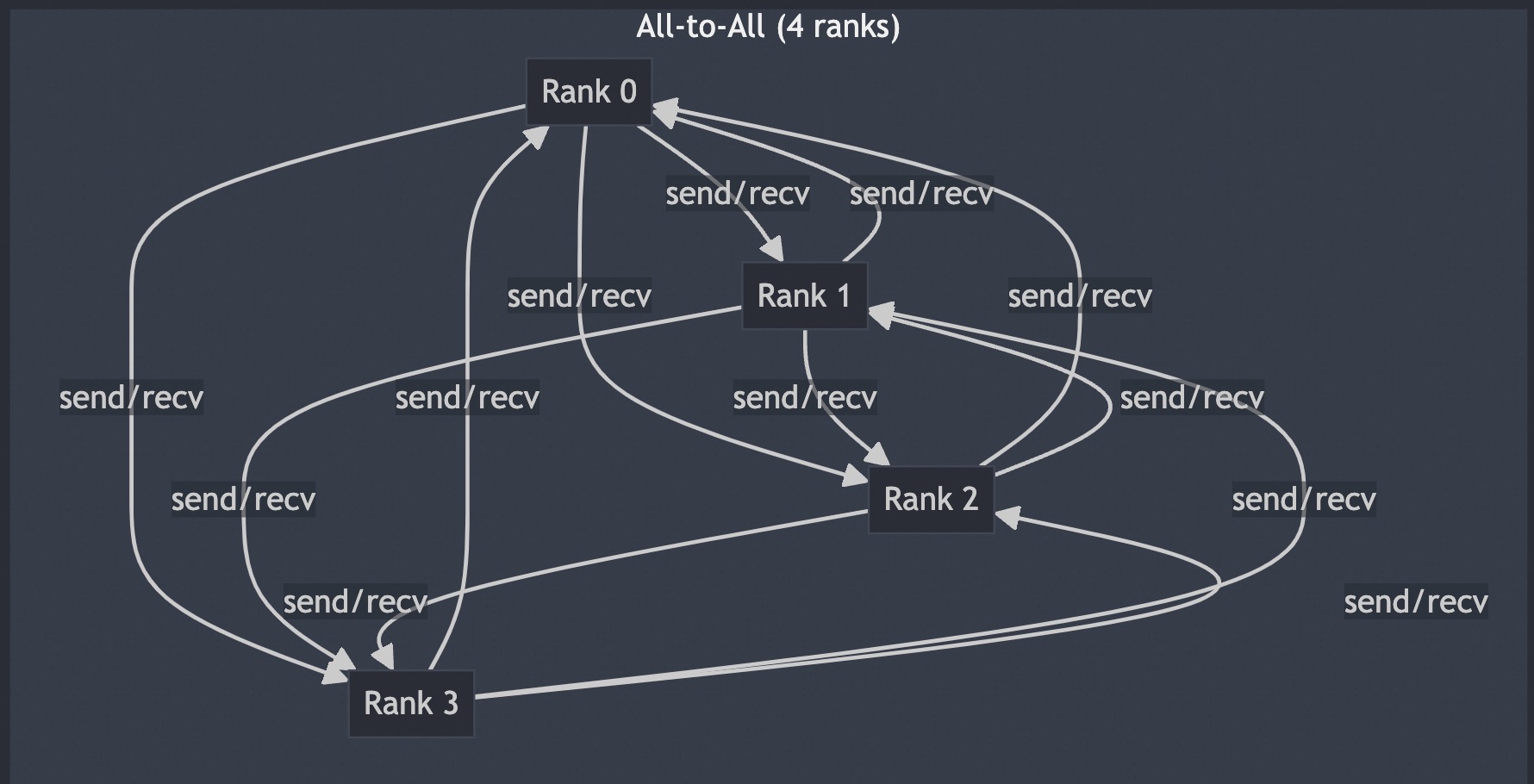
Alltoall 作用:每个进程向其他所有进程发送不同的数据块,同时从所有进程接收对应的数据块。其本质是全局数据重组(如矩阵转置)。Alltoall 是 Scatter 和 Gather 的组合,先 Scatter,再 Gather。
在 mpi4py 中,有以下三种类型的 Alltoall 集体通讯。
- comm.Alltoall(sendbuf, recvbuf)
- comm.Alltoallv(sendbuf, recvbuf)
- comm.Alltoallw(sendbuf, recvbuf)
comm.alltoall 方法将 task j 的中 sendbuf 的第 i 个对象拷贝到 task i 中 recvbuf 的第 j 个对象(接收者收到的对象和发送者一一对应,发送者发送的对象和接收者一一对应)。
下图可以表示这个发送过程。
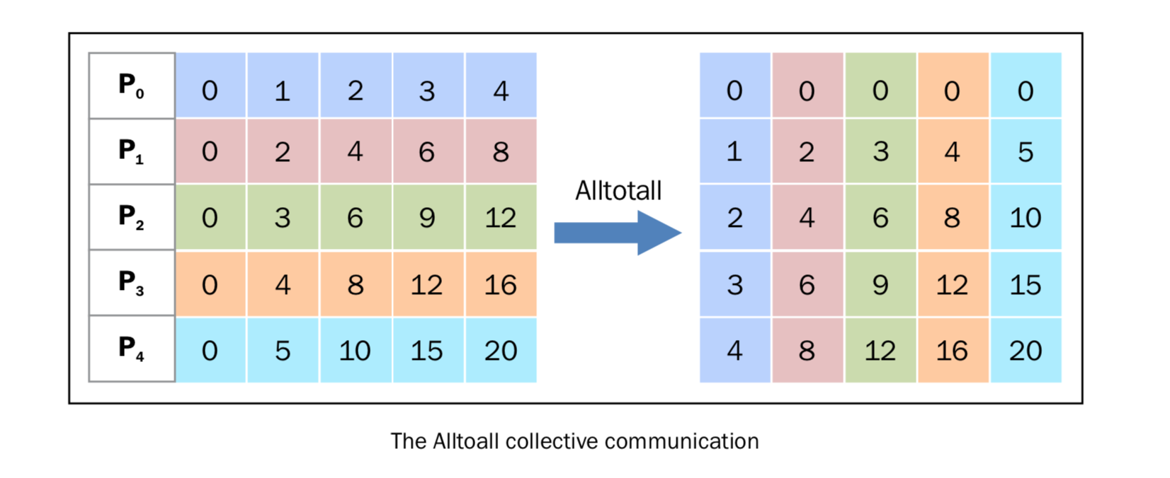
从发送和接收的接收的角度来理解,4个 rank 的 alltoall 的可视化过程如下图:
实例代码:
# alltoall_equal.py
from mpi4py import MPI
import numpy as np
comm = MPI.COMM_WORLD
rank, size = comm.Get_rank(), comm.Get_size()

# 准备发送缓冲区:一个二维数组 shape=(size, k)
k = 2
sendbuf = np.arange(rank*size*k, (rank+1)*size*k, dtype='i').reshape(size, k)
# 发送给自己的那一行可用作“自环”数据
print(f"Rank {rank} sendbuf=\n{sendbuf}")

# 预先分配接收同形数组
recvbuf = np.empty_like(sendbuf)
comm.Alltoall(sendbuf, recvbuf)

print(f"Rank {rank} recvbuf=\n{recvbuf}")
运行命令:
mpiexec -np 4 --allow-run-as-root python mpi4py_alltoall.py
输出结果:
Rank 0 sendbuf=
[[0 1]
 [2 3]
 [4 5]
 [6 7]]
Rank 1 sendbuf=
[[ 8  9]
 [10 11]
 [12 13]
 [14 15]]
Rank 3 sendbuf=
[[24 25]
 [26 27]
 [28 29]
 [30 31]]
Rank 2 sendbuf=
[[16 17]
 [18 19]
 [20 21]
 [22 23]]
Rank 2 recvbuf=
[[ 4  5]
 [12 13]
 [20 21]
 [28 29]]
Rank 0 recvbuf=
[[ 0  1]
 [ 8  9]
 [16 17]
 [24 25]]
Rank 3 recvbuf=
[[ 6  7]
 [14 15]
 [22 23]
 [30 31]]
Rank 1 recvbuf=
[[ 2  3]
 [10 11]
 [18 19]
 [26 27]]